Welcome to the tutorials section.
While a large portion of the site offers tips and info about various things that can help you save money, time, or enlighten you on things, this section is dedicated to learning new traits that can help you make money.
Learning/advancing through Excel, Are you proficient in excel, know just enough to get by, or have no knowledge of it at all but you want to learn? You are in the right place.
Excel spreadsheets are everywhere. You can use them around the home just as easily as at work for budgeting your own bills, keeping an index of things, or worksheets for various things. These walk-throughs can be found online anywhere from $20-$500 depending on where you go and it pays for itself considering the time it saves you in the long run and the money you can make from it by saving other’s time.
- Level 1- Beginner; Learn basic navigation, controls, tools, formatting, proofing, conditional rules, sorting, expanding, moving rows/columns, hidden comments and some basic formulas
- Level 2- Intermediate; Learn to create tables, charts, and conditional formulas & formatting
- Level 3- Advanced; Learn Pivot tables, drop down lists, and macros
Welcome to EEF Excel tutorial
This course is split in 3 levels; Beginner, Intermediate, Advanced. Each level will have 3-5 steps
If you are here, chances are you already know excel is a great tool to have, you just need a better understanding of it, so let’s dive right in.
Note: This course was made using Excel 2016, a lot of features can be used in older versions but some may only be accessed with 2016.
If you have any questions, comments, or suggestions along the way, please feel free to e-mail me at Ben@Eagleyeforum.com
GETTING STARTED
After this step you will be more comfortable with getting to know your keyboard shortcuts, understanding the main page and tab, and knowing the icons.
First, let’s go over shortcut buttons and function keys that make everything a little easier
| BASIC FUNCTION KEYS | |
| F1 | EXCEL HELP PANE |
| F2 | EDIT ACTIVE CELL |
| F3 | PASTE NAME (IF NAMES ARE DEFINED) |
| F4 | REPEATS LAST COMMAND |
| F5 | OPENS “GO TO” DIALOG BOX |
| F6 | SWITCH BETWEEN WORKSHEET, RIBBON, TASK PANE, AND ZOOM CONTROLS |
| F7 | CHECK SPELLING |
| F8 | EXTEND MODE |
| F9 | CALCULATE ALL WORKSHEETS |
| F10 | TURN KEY TIPS ON |
| F11 | CREATE CHART OF DATA IN RANGE ON NEW SHEET |
| F12 | SAVE AS BOX |
| BASIC CTRL AND ALT COMBO SHORTCUTS | |||
| CTRL + A | HIGHLIGHT EVERYTHING | CTRL + ` | COPY FORMULA FROM CELL INTO BAR |
| CTRL + O | OPEN WORKBOOK | CTRL + ‘ | COPY ABOVE CELL TO THIS CELL |
| CTRL+ W | CLOSE WORKBOOK | CTRL + SPACEBAR | SELECT ENTIRE COLUMN |
| CTRL+ N | NEW WORKBOOK | CTRL + F1 | SHOW/HIDE RIBBON |
| CTRL +S | SAVE WORKBOOK | CTRL + F2 | PRINT SETUP |
| CTRL + C | COPY HIGHLIGHTED TEXT/IMAGE | CTRL + F3 | NAME MANAGER |
| CTRL + V | PASTE/INDENT TEXT/IMAGE | CTRL + F4 | CLOSE WORKBOOK |
| CTRL + X | CUT HIGHLIGHTED TEXT/IMAGE | CTRL + F5 | COLLAPSE WINDOW TO SMALLER VERSION |
| CTRL + Z | UNDO PREVIOUS ACTION | CTRL + F6 | MOVE TO NEXT WORKBOOK |
| CTRL + Y | REDO PREVIOUS ACTION | CTRL + F7 | MOVE COMMAND (WHEN NOT MAXED, ARROWS MOVE) |
| CTRL + P | CTRL + F8 | SIZE COMMAND FOR BOOK | |
| CTRL + E | INVOKE FLASH FILL | CTRL + F9 | MINIMIZE WORKBOOK |
| CTRL + K | INSERT HYPERLINK | CTRL + F10 | EXPAND/RESTORE WINDOW |
| CTRL + L OR T | CREATE TABLE | CTRL + F11 | OPEN MACRO SHEET |
| CTRL + B OR 2 | BOLD FONT ON/OFF | CTRL + F12 | OPEN WORKBOOK |
| CTRL + U OR 4 | UNDERLINE FONT ON/OFF | ALT + H | HOME TAB |
| CTRL + I OR 3 | ITALIC FONT ON/OFF | ALT + N | INSERT TAB |
| CTRL + 9 | HIDE SELECTED ROWS | ALT + P | PAGE LAYOUT TAB |
| CTRL + 0 | HIDE SELECTED COLUMNS | ALT + M | FORMULAS TAB |
| CTRL + HOME | MOVE TO BEGINNING OF SHEET | ALT + A | DATA TAB |
| CTRL + END | MOVE TO LAST CELL WITH CONTENT | ALT + R | REVIEW TAB |
| CTRL + PAGE UP | MOVE TO NEXT SHEET | ALT + W | VIEW TAB |
| CTRL + PAGE DOWN | MOVE TO PREVIOUS SHEET | ALT + L | DEVELOPER TAB |
| CTRL + 1 | ALT + Y | HELP TAB | |
| CTRL + 5 | APPLY OR REMOVE STRIKETHROUGH FONT | ALT + B | ACROBAT TAB |
| CTRL + 6 | SWITCH BETWEEN HIDING OBJECTS | ALT + Q | TELL ME/SEARCH TAB |
| CTRL + 8 | SHOW/HIDE OUTLINE SYMBOLS | ALT + 1 | SAVE |
| CTRL + ~ | SHOW/HIDE VALUES AND FORMULAS | ALT + 2 | UNDO |
| CTRL + – | DELETE CELL(S) | ALT + 3 | REDO |
| CTRL + ; | TODAY’S DATE | ALT + ZS | SHARE |
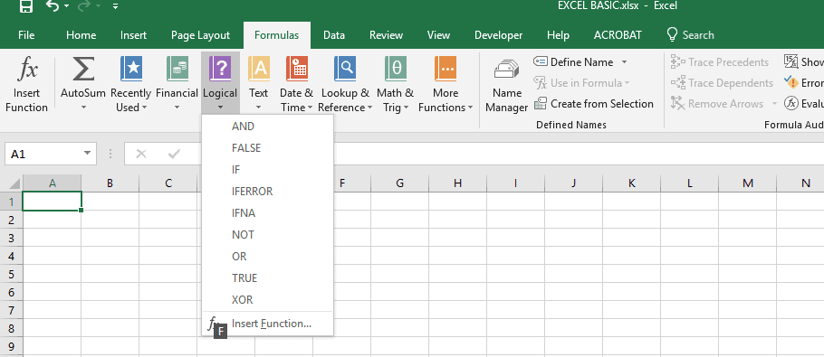
While you need to hold “CTRL” with the character for those to work, the “ALT” command just needs to be pressed which will open up a list of characters over areas that can be pressed by key board to access;
If I were to just press “M” after this, it would take me to the “Formulas” tab where everything is still highlighted with quick access;
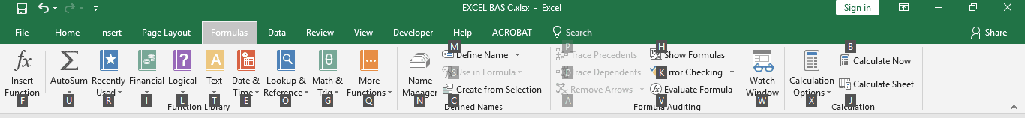
Now, if I were to press “L”, it would drop down the list of functions instead of having to drag and click with a mouse
Now, let’s go over your workbooks once you open it;
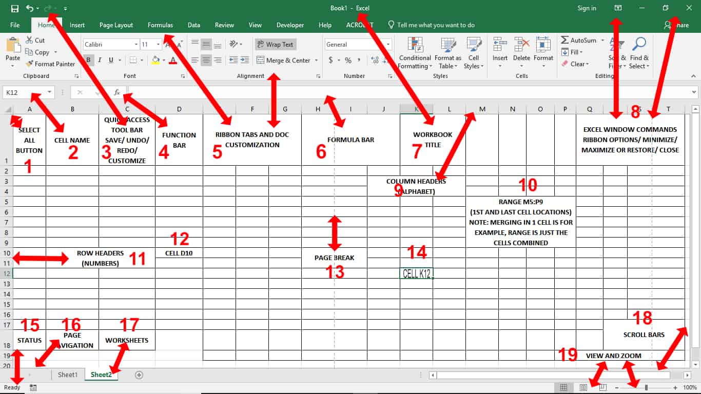
- Select all button; Highlights the whole page, even what you have not written on. Quick for setting everything the same font, size, positioning, etc.
- Cell name; the name of the cell you are on.
- Quick access toolbar; From left to right we have the save icon, undo arrow to change your last change (CTRL+Z), redo arrow (CTRL+Y), and customization.
- Function bar where you can look for types of formulas and input them
- Ribbon tabs and document customization bars; the tools to do the job
- Formula bar; what’s written in each cell can be seen here, formulas included
- workbooks title
- Excel window commands
- Column headers (A,B,C, etc.)
- Range: highlighting cells (like M5 to M9 in the example) is called a range
- Row headers (1,2,3,etc.)
- Cell D10
- Page break is where it will cut off if you print the sheet
- Cell K12
- Sheet status (ready, edit, saving, etc.)
- Page navigation to easily travel through your workbooks sheet
- Titles of worksheets in your book
- Scroll bars
- View and zoom controls
Note: In excel a quick navigation from cell to cell is your up, down, left, and right arrows, if at any point they don’t work, check your “scroll lock” button on your keyboard.
Speaking of navigation, besides your standard mouse arrow, here are other icons that you may see as you scroll over parts
![]()
BASIC FORMATTING AND RULES
After this step, you will be more comfortable with the HOME tab, as well as utilizing universal rules, basic format cells dialogue box and sorting, filtering, finding, and replacing content
Now let’s look at the “FILE” tab;
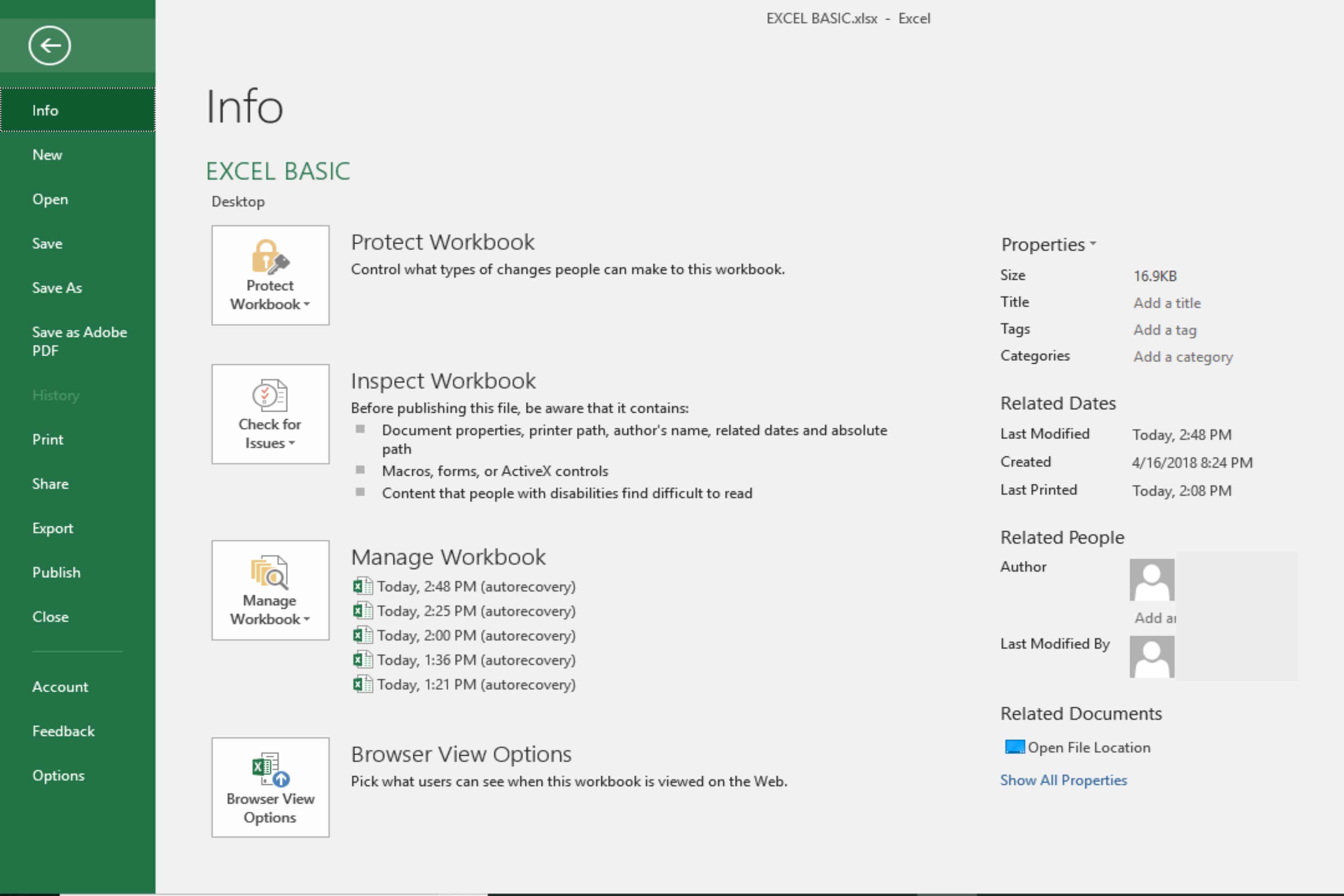
Once opened, you will notice it is on the info tab. Here you have options of protecting your workbooks with a password (which can also be done on the main page but we will get to that later), managing, inspecting, and even what you are willing to share online with the browser view options. To the right we have the property areas where you can edit the title, tags and categories and see the size and important dates and people regarding the file.
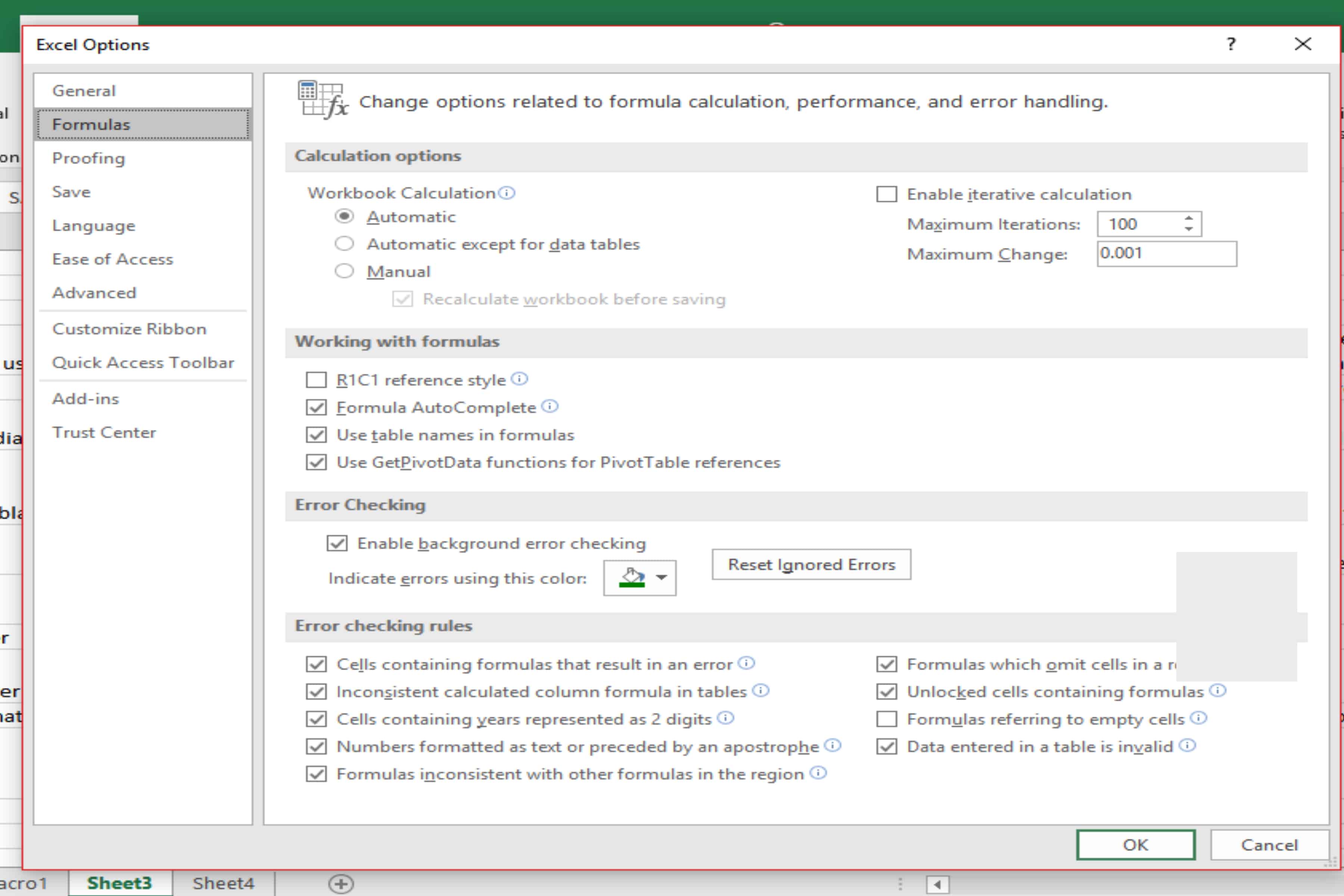
All the other tabs are pretty self-explanatory but options opens up tabs of basic procedures you want it to do universally;
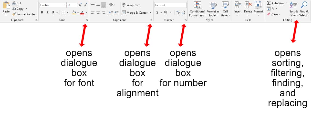
Back to our main page, if you right-click anywhere on the sheet and click “format cells” it opens a dialog box for the “HOME TAB” tools, some are also found on the ribbon and accessed via the “dialogue box”, also referred to as the “more” button;
First tab in the format cells menu is “NUMBER”

- General is the data as is
- Number gives you options of adding decimals and “,” when 1,000’s occur
- Currency adds the $ sign to numbers
- Accounting puts that dollar sign fixed to the beginning of the cell to give the number space.
- Date allows you to format how dates appear
- Time allows you to format how time appears
- Percentage converts your number to a percentile
- Fraction converts your number to a fraction
- Scientific helps with math formulas
- Text is data as is
- Special can be used for specific formatting on phone numbers, zip codes, and SSN where “-” are used
- Custom gives you a wide range of all the above and then some
Second is “ALIGNMENT”
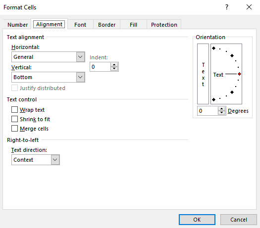 Here is pretty straight forward on how to align your text in reference to your cell as well as some text control;
- Wrap text will allow words to flow below, extending the row height instead of column width, if you want shorter column widths
- Shrink to fit does just that, shrinks your text to fit
- Merge cells allows you to merge highlighted cells where the 1st cell information takes over and deletes all the rest.
- Text direction is reading left-right or right-left
Third is “FONT”
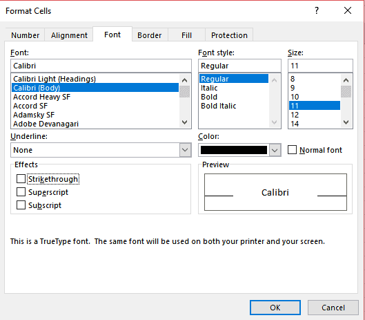 Font gives you a preview of your selections. You can range in type of font, style, size, color, and effects.
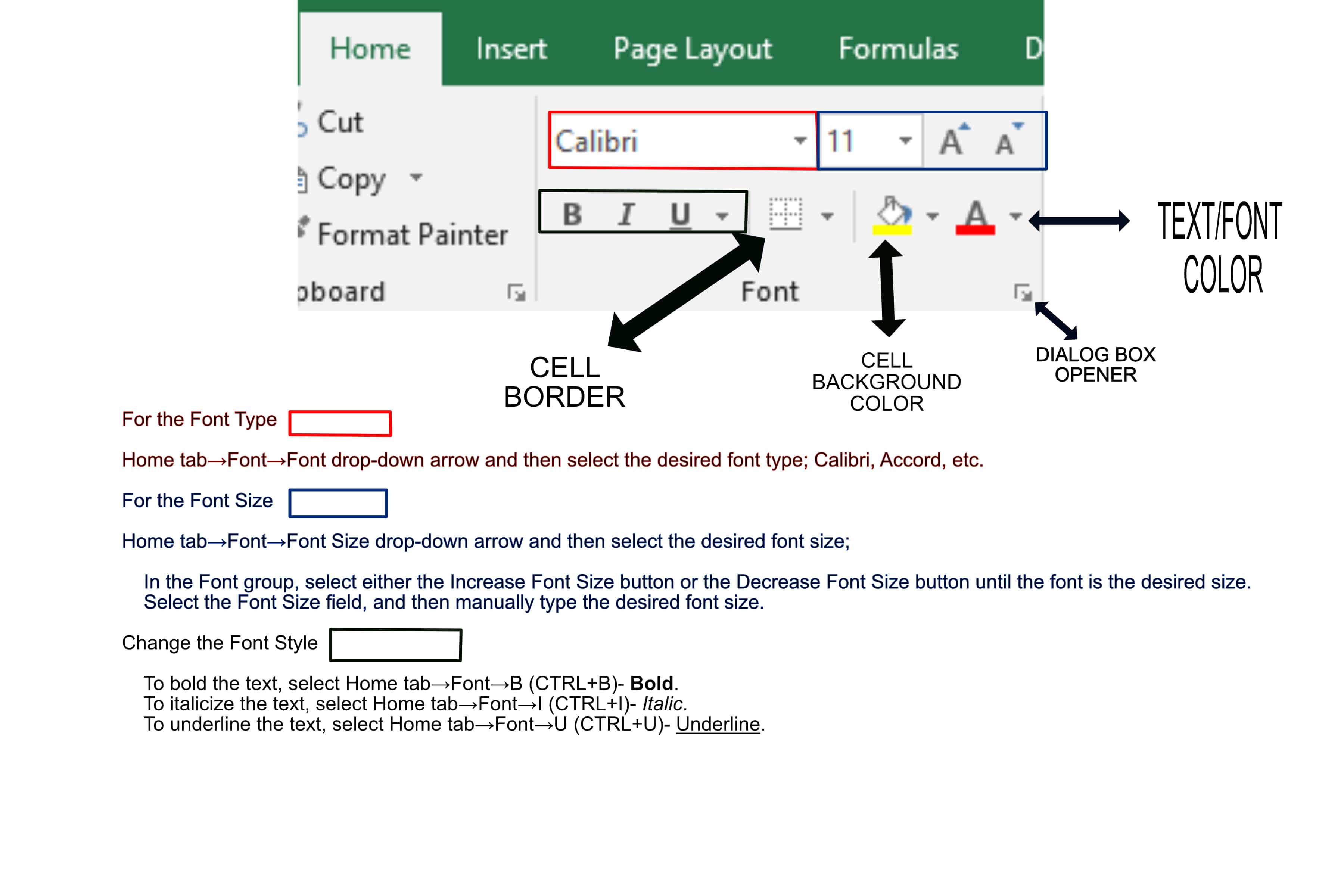
Use the Format Cells Dialog Box to Format Text
Home tab→Font→dialog box launcher.
In the Format Cells dialog box, ensure that the Font tab is selected and configure the desired font formatting and then select OK.
To change font from the main page, select the desired cell or range;
Fourth is “BORDER”
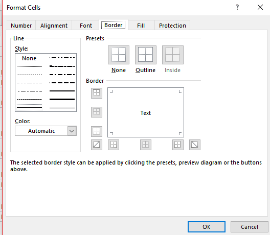 Border is where you can darken cell or range outlines to distinguish different areas, especially in printing. Leaving the sheet with a normal grid and printing it, shows no grid.
You have the options of style, presets, and color, and border;
- STYLE gives you dotted, straight, and a mix of both
- PRESETS allows you to fill the outline or inside cross as a whole of whichever style you chose.
- COLOR changes the border color
- BORDER allows you to just pick single walls, inside, outside , or diagonally
Fifth is “FILL”
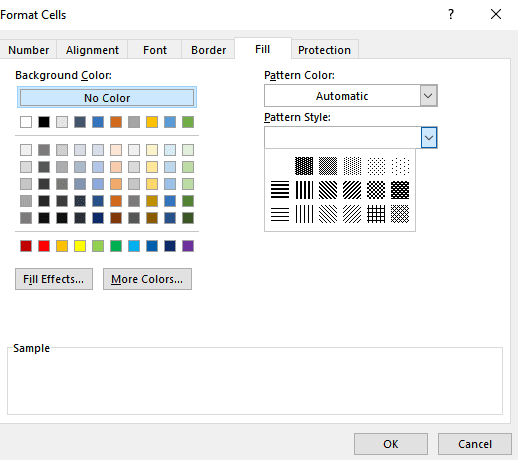
Last important one is “FILL” where you can color in the background of cells, add patterns, and add effects.
The protection tab is for protecting sheets and formulas, you will learn more about those later when its applicable.
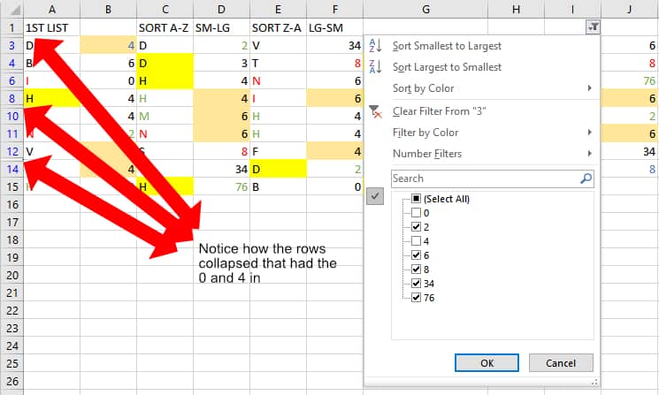
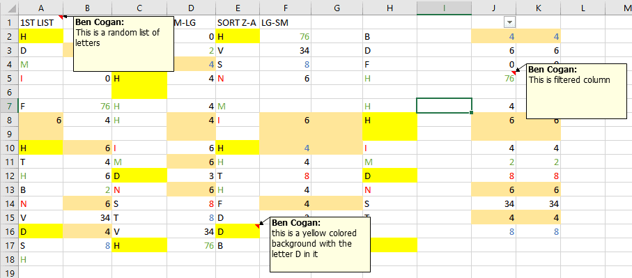
Here is a little breakdown of sorting, filtering, finding and replacing;
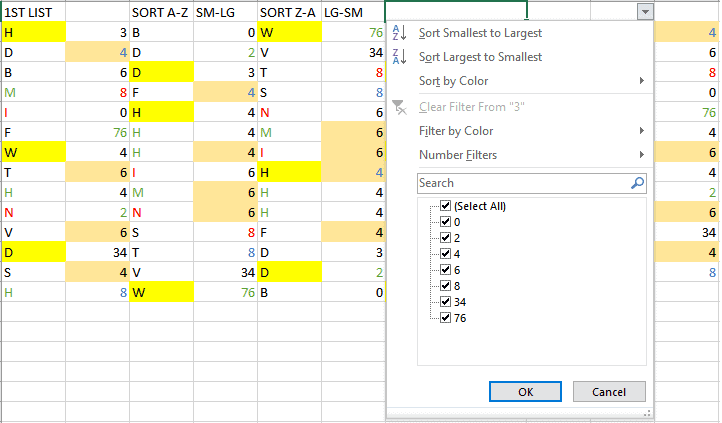
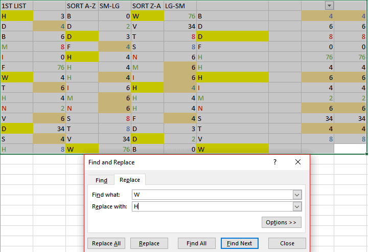
Notice that the 1st 2 columns are what I put in originally, the next 2 were highlighted and sorted by A-Z and small to large, the next 2 were highlighted and sorted Z-A and large to small. The last one is set on filter, it drops a list of the cells and you can uncheck them to hide them, but they will hide everything on their row.
There is also a custom option where you can add levels for multiple sorts and set them in an order of which takes precedence first;
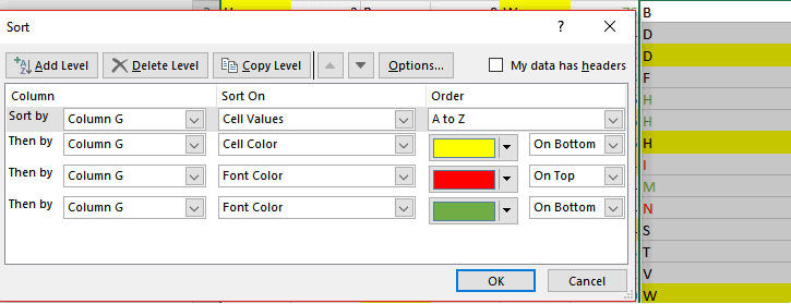
These are set by A-Z first, then if multiples are present, the yellow background types would sit on the bottom of that group, then red font sitting on top, followed by green font sitting on bottom.
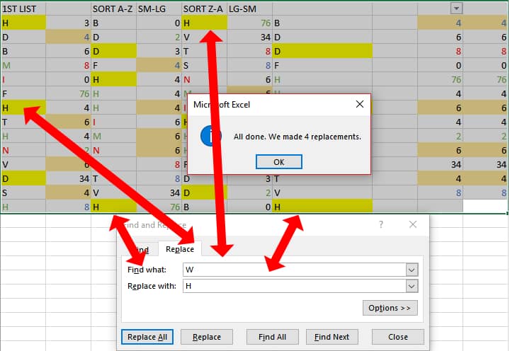
Now to find and replace characters;
Once I hit replace all, I get all 4 W’s changing to H’s
PROOFREADING, ADJUSTING AND COMMENTS
After this section you will be more comfortable with the REVIEW tab, as well as;
- Moving cells, rows, and columns around
- the Proofing of your work
- Adding hidden comments to cells
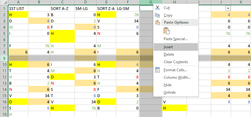
Depending on what you are doing, you may need to move things around at some point, you can do this by highlighting your cells, rows, and columns
Once you have the cell, row, or column highlighted, “right-click” on the mouse, click “cut”, then move over to the area you want it, right-click and “insert cut cells”. Wherever you drop your cell and row, it will take the number/letter of the row/column in front of it. When moving a cell, it will give you a message of whether you want to move the cell you are inserting into, to the left, right, up, or down.
You can move a groups of rows, columns, and even cells but you can’t mix them up or grab them at random spots, they have to be together.
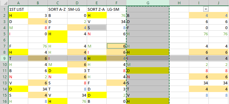
You can also insert new columns and rows in between work
If you have a lot of text in your worksheet that you need to spell check, you can do so by hitting the “Review” tab
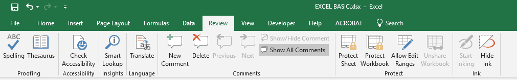
Here I put the pledge of allegiance on my excel sheet and added a bunch of typos, then hit the spell check located on the far-left of the ribbon where it hits on the 1st misspelled word and gives you alternatives;
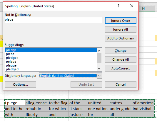
You are then given the options to ignore if you know the spelling is correct (like last names, company names, etc.), look and change each word, or just trust the spell check to change them all, I am going one by one and making a note here;
notice that it passed up “it stans” instead of stands, this is where it can get deceiving because although you meant stand, it recognizes “stans” as a plural of the word stan, which has a meaning in some, if not all, dictionaries.
Case in point: While spell check is a great tool, don’t expect it to fix all of your mess-ups
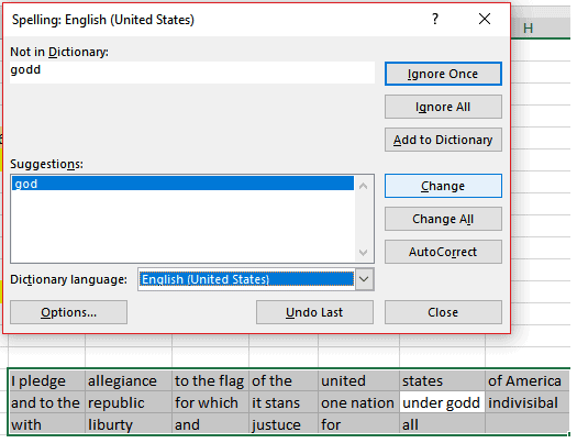
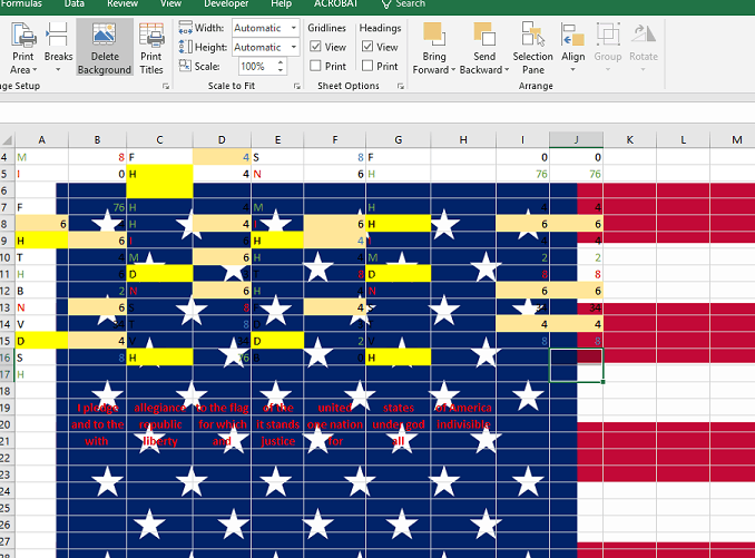
Now, just for giggles I jumped into the Page Layout tab and added a background to my sheet to go along with the pledge;
You can also add comments to cells, this helps especially for shared worksheets where you want to hide info about your sheet but still show others what you did;
Now for what Excel is best for;
BASIC FORMULAS
After this section, you will be more familiar with basic formulas from the “Formula” tab, such as;
- Basic math formulas (Add, subtract, multiplication, and division)
- Finding averages
- “COUNTIF” formulas
- Tip / commission calculator
Here we have a simple spreadsheet loaded with basic formulas;
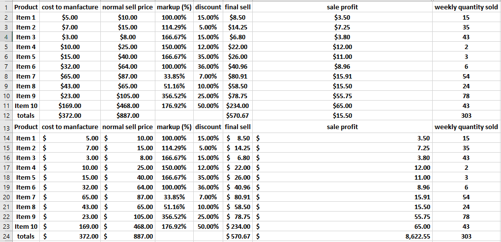
They were duplicated so that you can see them easier on this next image when the formula is shown (CTRL+~);
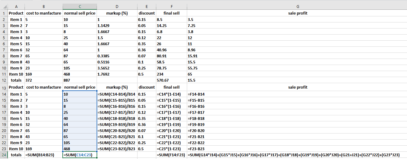
Note: When you are in “show formula” mode, you can click on the formula to see the cells affected as shown.
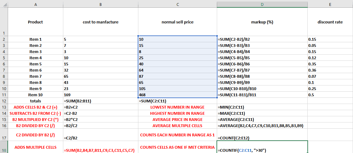
Here is a simpler sheet with descriptions of what it is being asked to do;
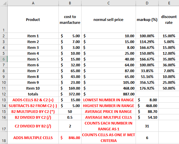
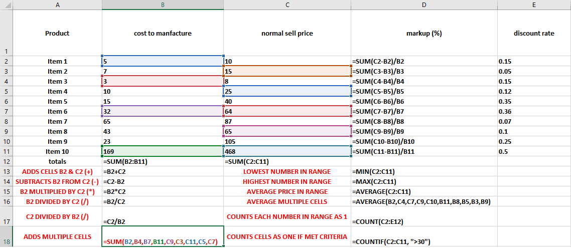
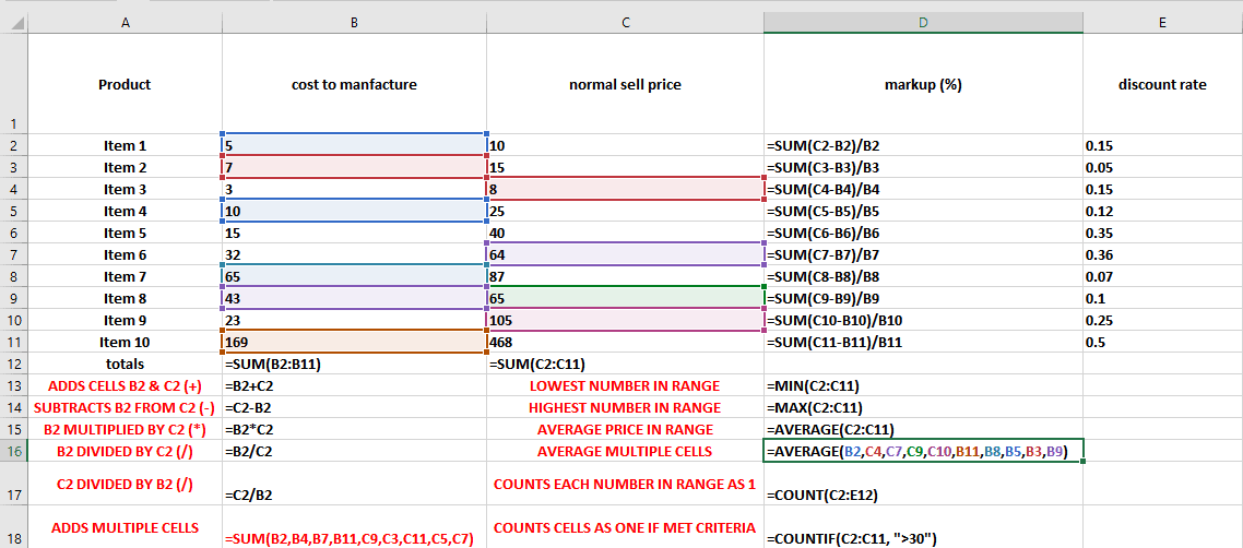
If you can’t guess which cells are affected, here are a few more with breakdowns of each type;
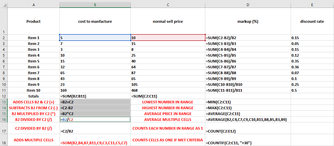
Notice B13-B17 are all playing off the same cells. The same is done here for finding the sum (C12), minimum number (D13), maximum number (D14), and average (D15);
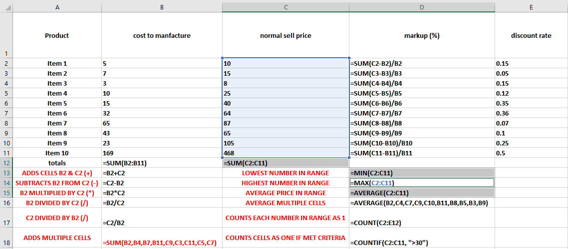
When looking for a sum or average, you do not need to stay in range or group, you can click your 1st cell, then hold “CTRL” and click on all the other cells you want in the equation
A couple other basic formulas that some people use often is “COUNT” and “COUNTIF” which as shown in descriptions, they count 1 for every cell shown if it shows content or meets criteria;
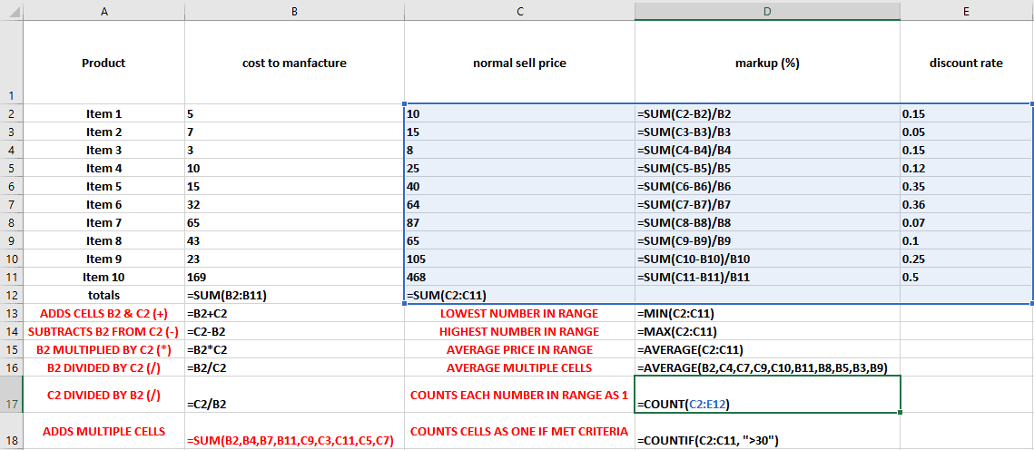
Notice the count only added 31 to D17, it did not add 1 for the two blank spaces.
I have directed “COUNTIF” to count only ones greater than 30, quotations are important here when giving a command, this could have been any number, or even cell. If you wanted to add greater/lesser than or equal to, you would need to form it like this; (“>=30”, “<=30). Equals (=) starts the equation so you can’t start a second one with it already in one which is why the “<>” come before the “=”, not after.
NOTE: When creating formulas, you can manually type them in the formula bar, go through the formula tab and follow prompts, and even just click cells after an “=” sign is added.
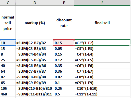
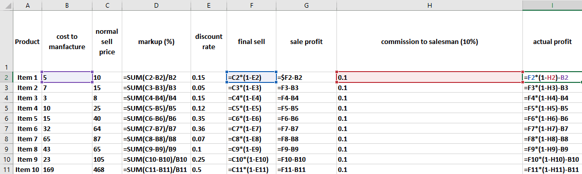
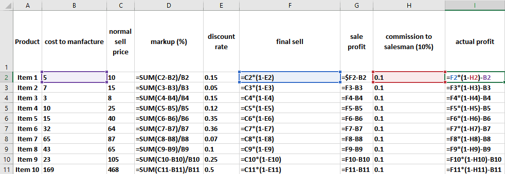
Now to get a little more complicated by throwing in percentages and fractions for calculating purposes, here is the full spreadsheet I made;
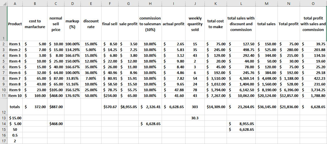
You have your “cost to make” and “normal sale price”, next to those it gives you the percentage of the markup and to calculate your discount you have;
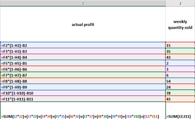
To get what the profit would have been without a sales commission, you would have;
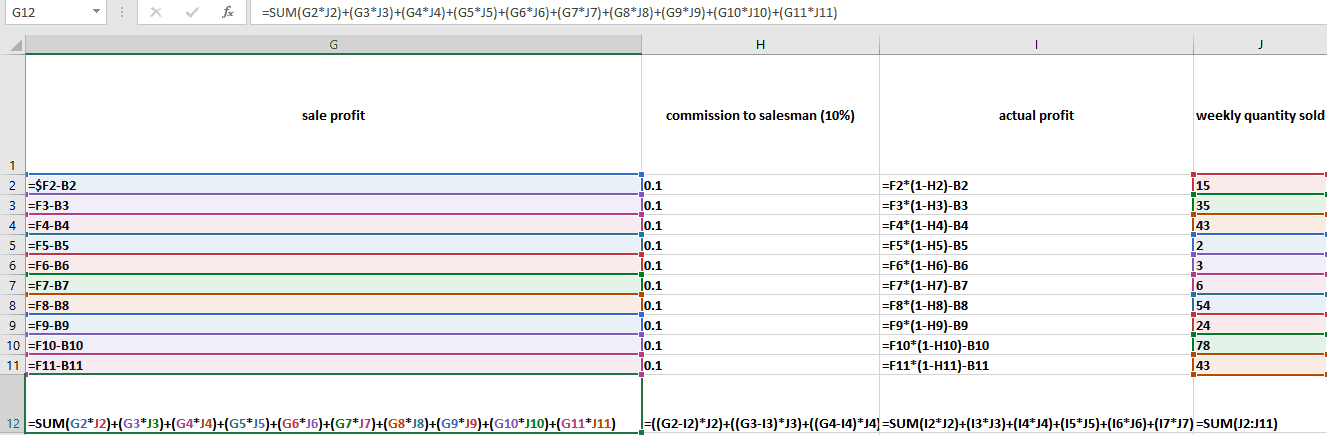
Now when you want to know how to calculate your salesman commission;
If you want to know how much your profit was after paying commission;
Here is if you want to find out how much your sales rep made overall;
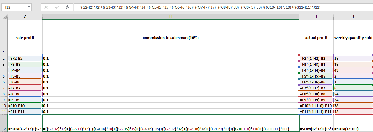
And your final profit after discount is applied and your commission is paid;
If you are looking for a tip calculator, the same types of formulas are applied, although in different order;
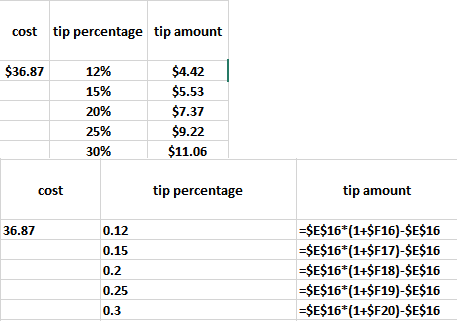
The “$” is referenced in the formula as an “absolute” command, it is used for quickly applying the same formula all the way down. The $ tells excel the cell stays the same. If you normally copy and past formulas, it goes in sequence as well, but this tells it to stay on the cell that has the value of $36.87 for E16 but count down on F16-20.
That does it for the basic course. By now you should be comfortable short-cutting and navigating around excel, understanding symbols, cleaning up your doc, organizing, expanding, formatting, and performing basic math equations. I hope this serves you well. Please let me know if you have any questions or suggestions about this page; Ben@Eagleyeforum.com
Next section we will cover more complicated conditional formulas, inserting tables and charts, flash filling, applying styles and themes, creating templates, working with functions, and querying data.
By now you should be pretty comfortable identifying key components of the User Interface and working with spreadsheets for basic formulating and formatting needs. Now lets dive a little deeper into tables, charts, conditional formulas & formatting, and if you have the 2013 or newer version; flash fill.
Flash fill
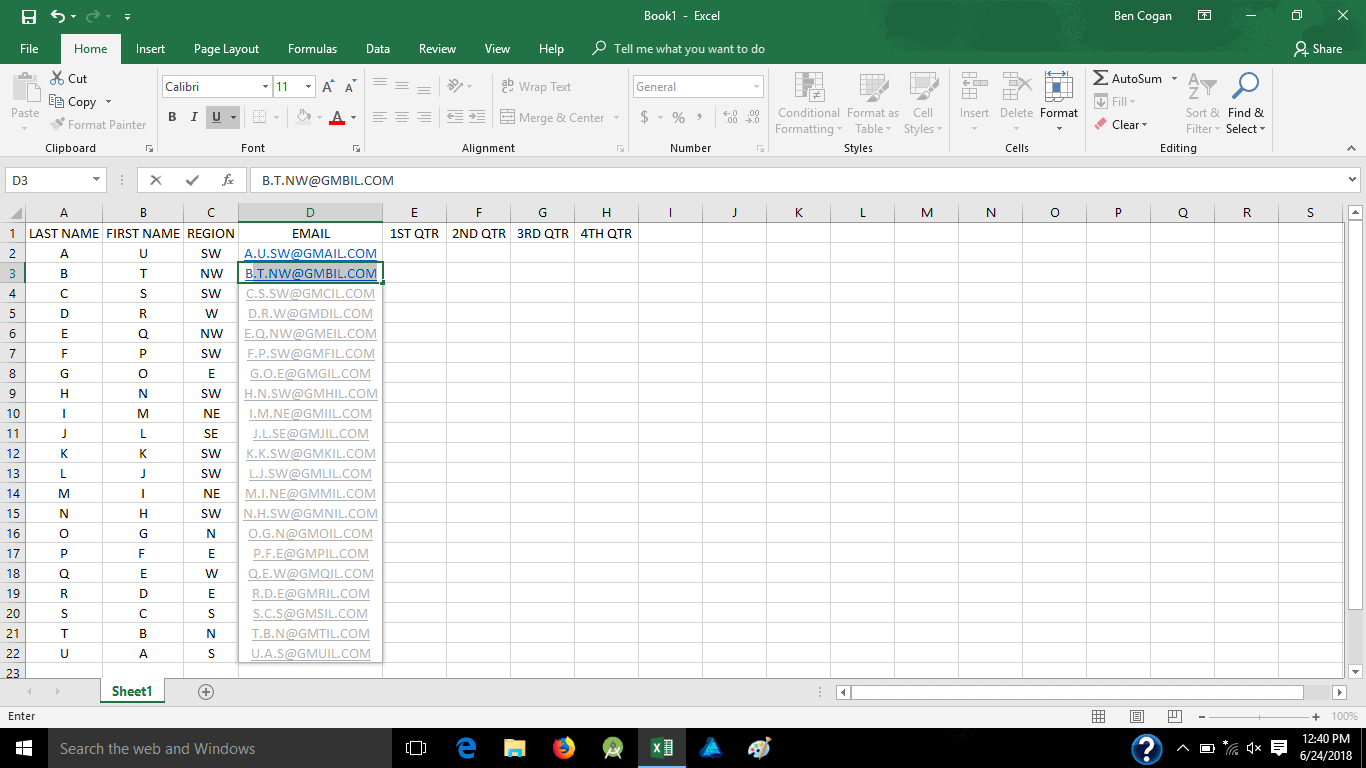
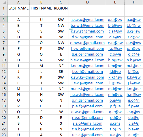
Flash fill is a great tool if you need to combine content from a few cells together separately for every row. You can find it on your quick format box or on the top right under editing. Here, you type in a couple of cells and it notices the pattern you are going for down the column and makes a suggestion, but the pattern box can mislead you, here I put letters of the alphabet as names, added region for where they are working and I want to get them all in an email list without typing in each one;
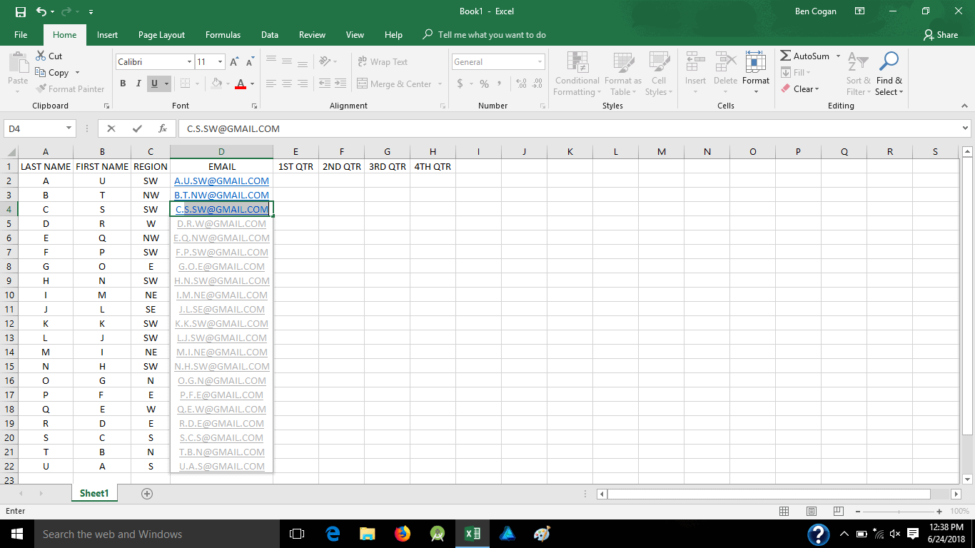
Notice how it picked up “Gmail” and counted the A in alphabetical order, that was while typing the second one so I manually punched it in too. If you accidentally hit the box and accept them all, you can easily press CTRL+Z to “undo” instead of deleting each one. Here is how it how it came out
You just need to stay in line, if you try doing it a column away, it won’t come through, you would have to type each manually, but when you stay in line you can go out-of-order on the content and mix it up, like this;
That’s flash fill, simple tool that can go a long way if you have a huge list you need to combine. Instead of the past wasting an hour or so typing in each one, now you can get it done in seconds.
Conditional format/formulas & working with tables
Now let’s throw out some numbers and add some formulas, conditional formatting, and some rules;
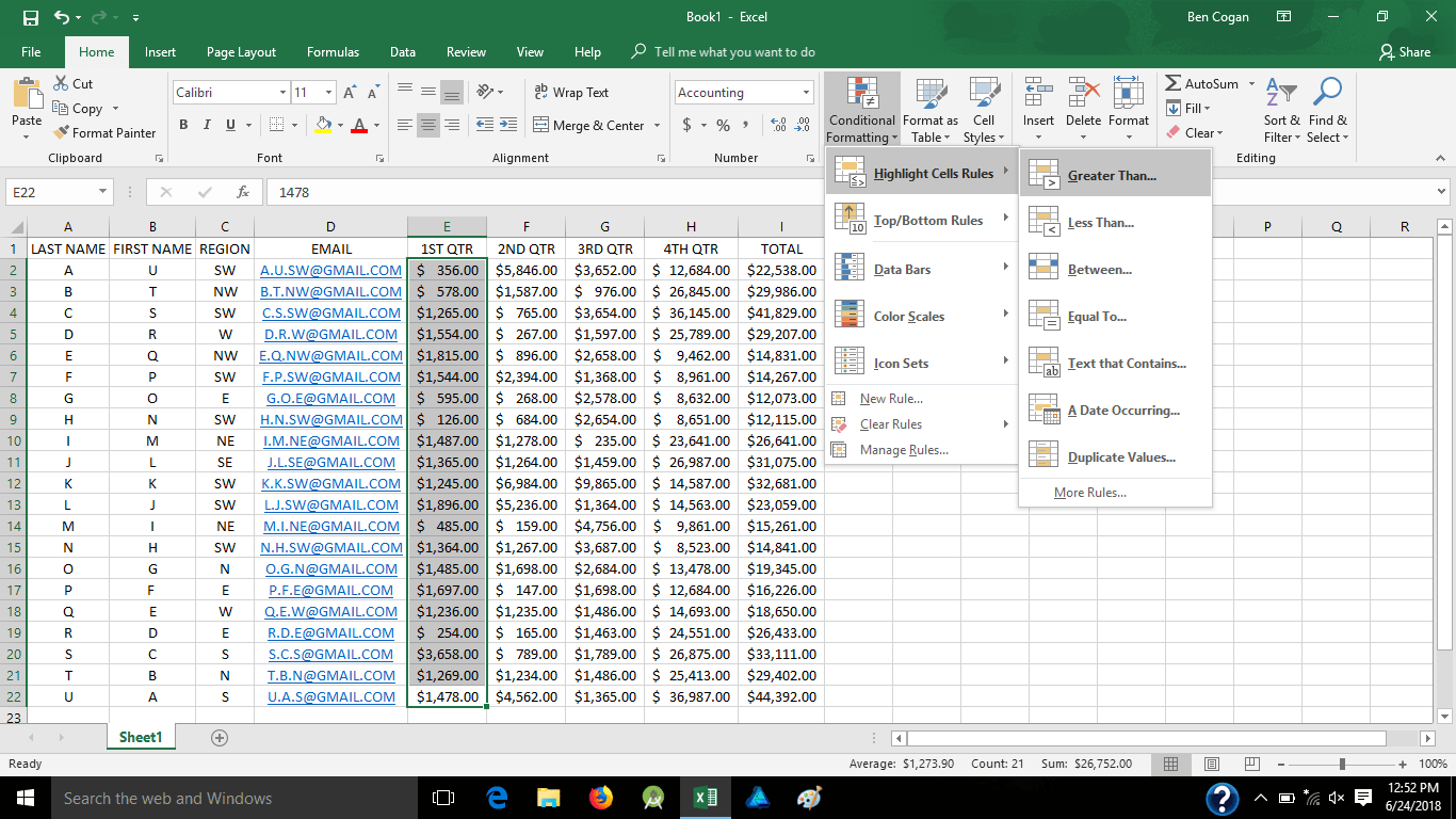
Picture this as a sales rep sheet providing their quarterly sales and annual totals, but it looks like a pain to differentiate cells, especially with a bigger list so lets set some formatting like inserting a new second row and adding monthly dollar figure goals, then I hid that row so it’s not distracting. Here we painted each cell green if it was over “$X” and red if it was under. Here were the values of each;
- 1st qtr greater than/less than $500
- 2nd qtr greater than/less than $1000
- 3rd qtr greater than/less than $2000
- 4th qtr greater than/less than $15000
- Total greater than/less than $25000
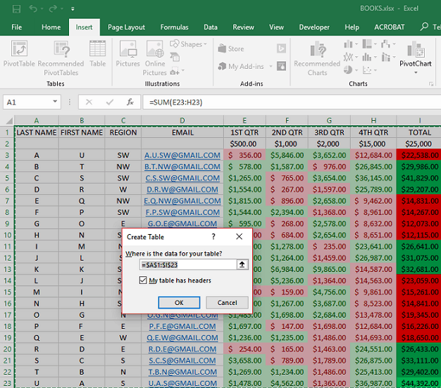
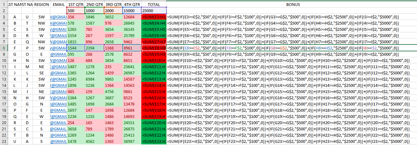
Let’s convert it to a table for easier sorting if necessary, here I also added a new 2nd row for sales rep bonuses. Highlight the whole area, insert table, confirm the data Excel picked as your data and go;
Now when in a table, there is a separate tools tab on the ribbon called “Design” when you go there you can change theme, style, and content of headers. You can see a chart on the upper right where you can change your table style. You can also see I added the bonus total, and some other conditional formulas for those sales reps.
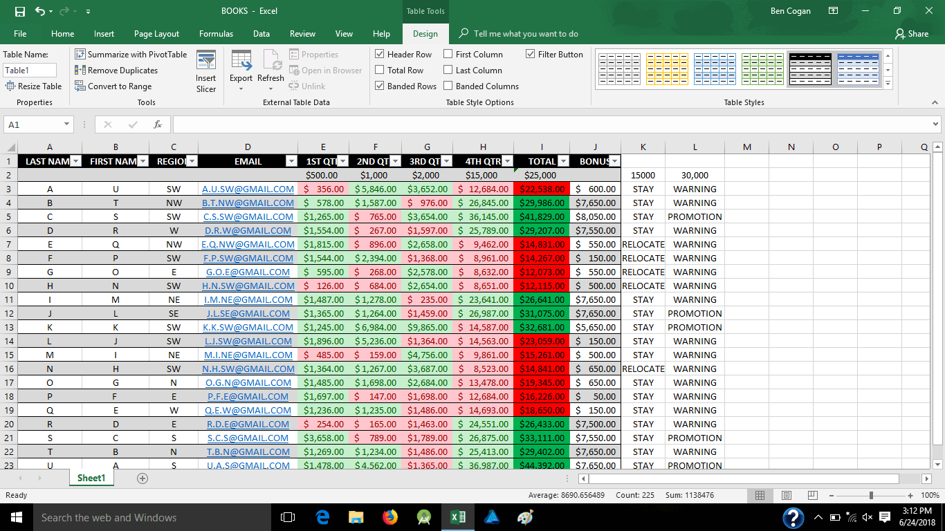
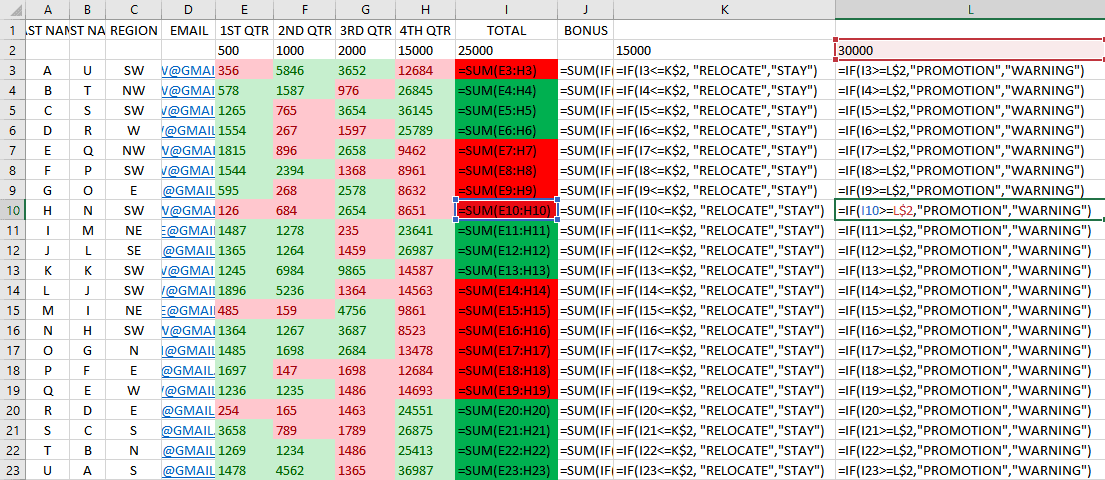
Bonuses are based off of their quarterly sales, the other conditional formulas indicate whether a sales rep did good or bad and will either be staying or relocating to a different region, and if they will receive a promotion or warning for their performance. Here are those formulas;
Now lets focus a little more on the table for easy sorting, here I’m clicking on the drop-down arrow of the “total” column;
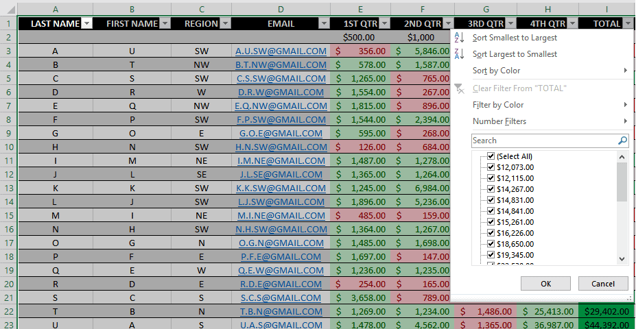
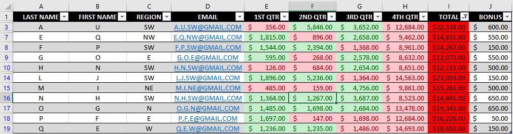
And we are going to sort by color, looking at only the lowest totals in red. You can play around with this and change by region, names, quarters, colors and even basic low to high/high to low numbers.
Charts
Now let’s add some charts to make it look a little better, highlight the area you want to chart out as well as the headers for the axis titles, then go to “insert” tab and click “recommended charts”
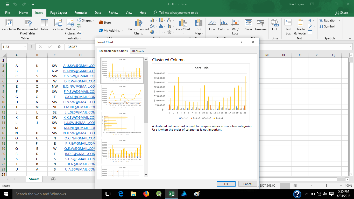
Here it will give you a list of charts it recommends will flow well with your data, we will just grab a simple bar graph, then pick the cell you want it to appear in;
And here it is;
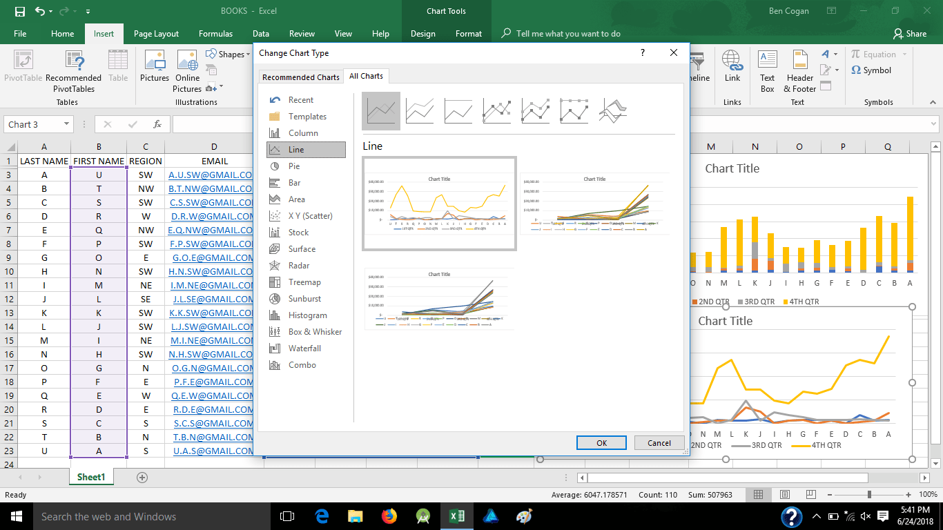
Now lets add another, this time a line chart;
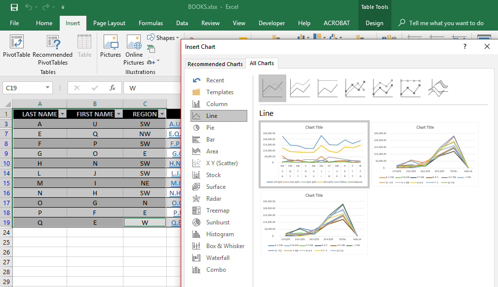
and place it, if prompted
Now you can click on the charts and edit the layout and/or title 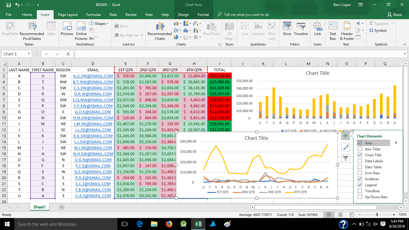
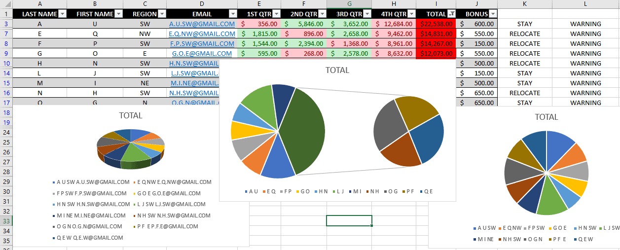
Here’s a few pie charts of the same data;
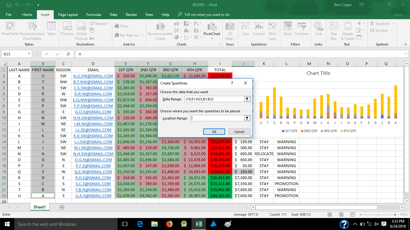
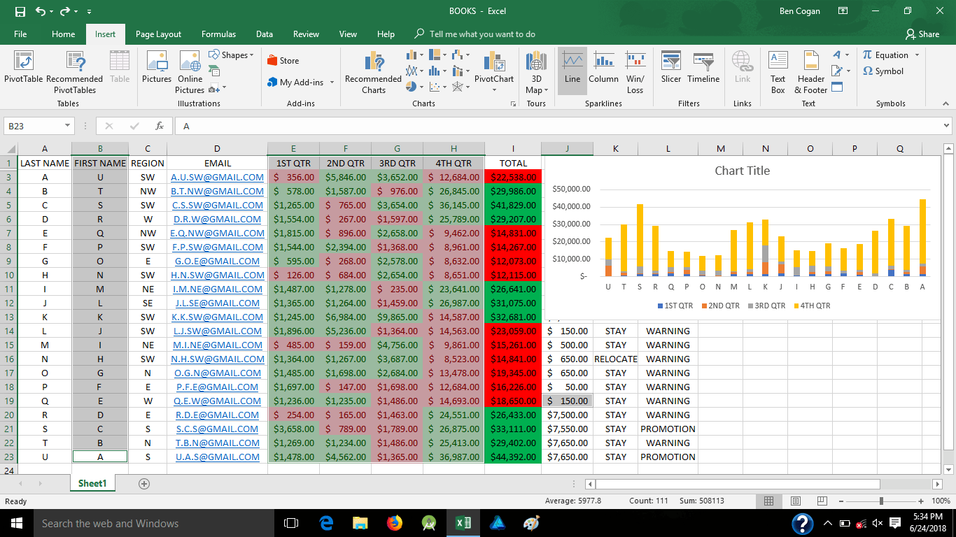
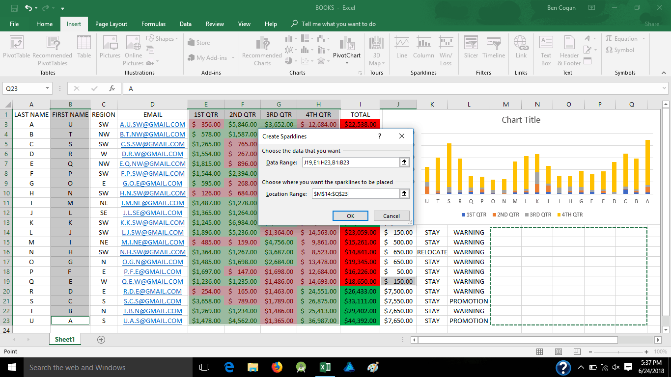
If you don’t like everything grouped together and just want a simple line chart for each person’s progress, you could easily do 1 for each line, just highlight the cells you want, add line chart (also know as spark-line) and place in the cell you wish them to go to;
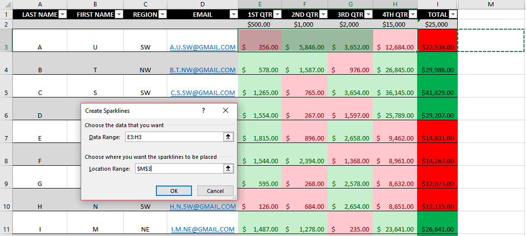
Now we add some style to it by coloring the line and marker points;
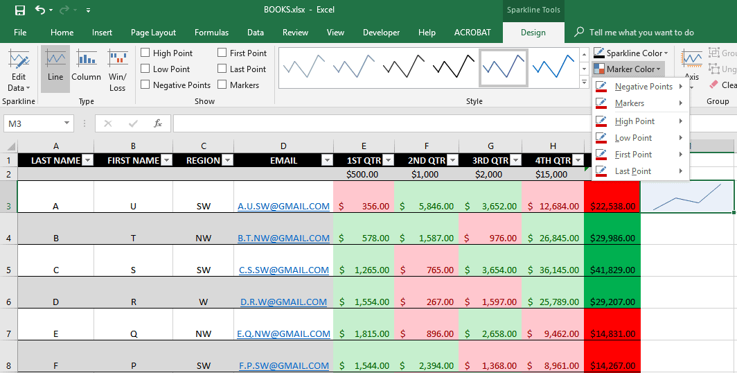
Notice that the “location range” when you pick where you want the line to go has the “absolute reference” ($), that means that once the line is set, if you go to the bottom right corner and use the black + symbol to copy it to the other cells, it will pick up the new data from each row, with markers;
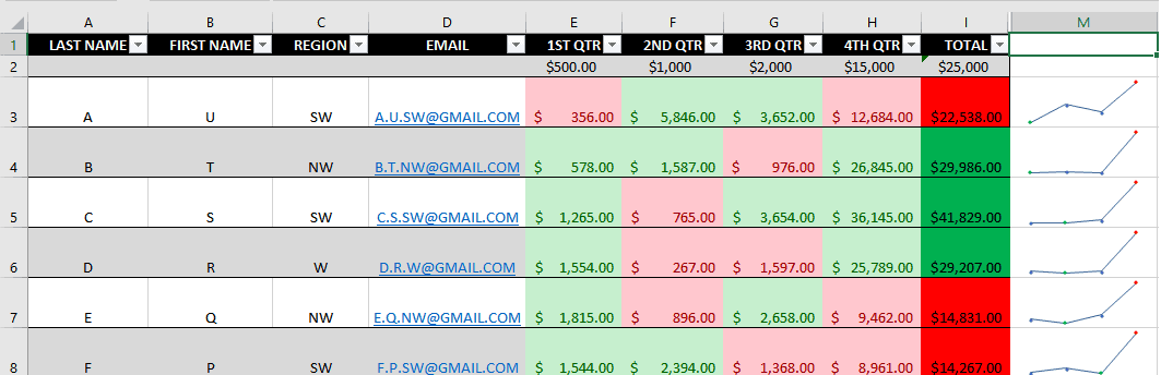
Just that easy.
Football Pool Formula
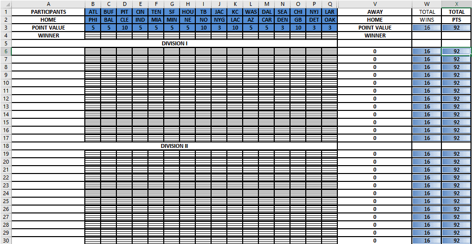
Now let’s get back to conditional formulas. I learned these the hard way many years ago creating football pools. It literally took me about 7 hours to create. This was also because I had no idea about the absolute reference, I manually punched the formula in 20 times before I even realized I could copy that formula to word 100 times, then find and replace each number with the next number in line… hence why it took 7 hours. Here is that football pool for your reference;
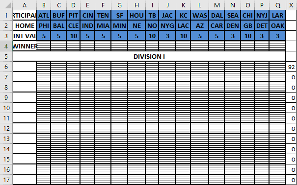
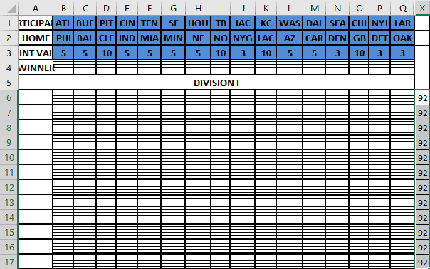
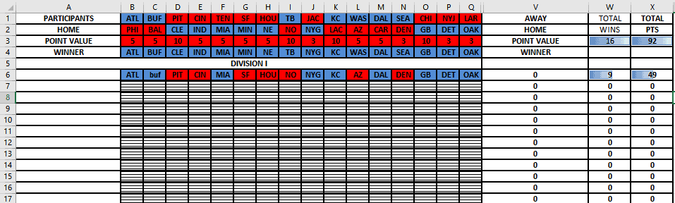
This is week 1 spreadsheet, there is a lot going on here from conditional rules, to conditional formulas, to even data point bars ranged so you can clearly see the difference between you and your opponents without looking at points tallied.
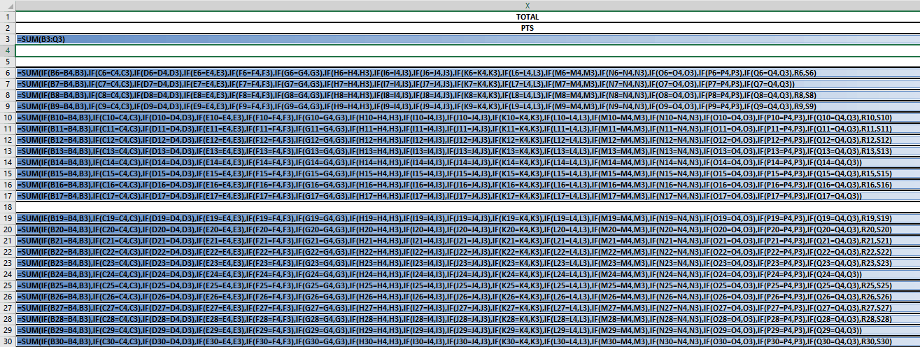
Here is the full formula for the total wins, (disregard the letters between Q and V, they were for a different format) this is my original formula, notice no “$” absolute references. This is how I got the 16 for total wins, 1 point for each game.
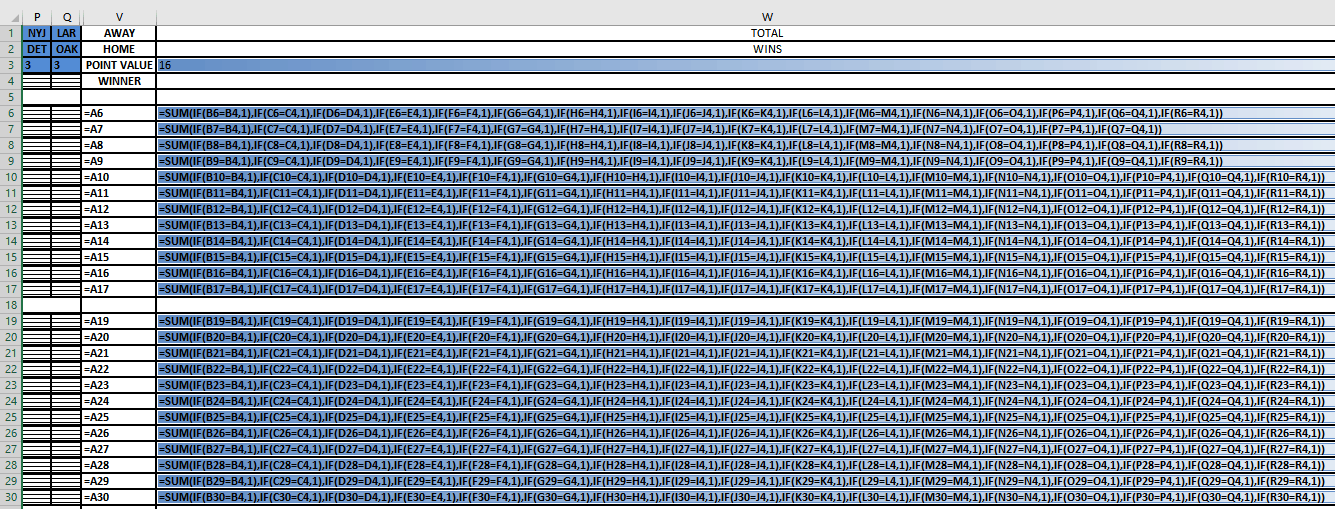
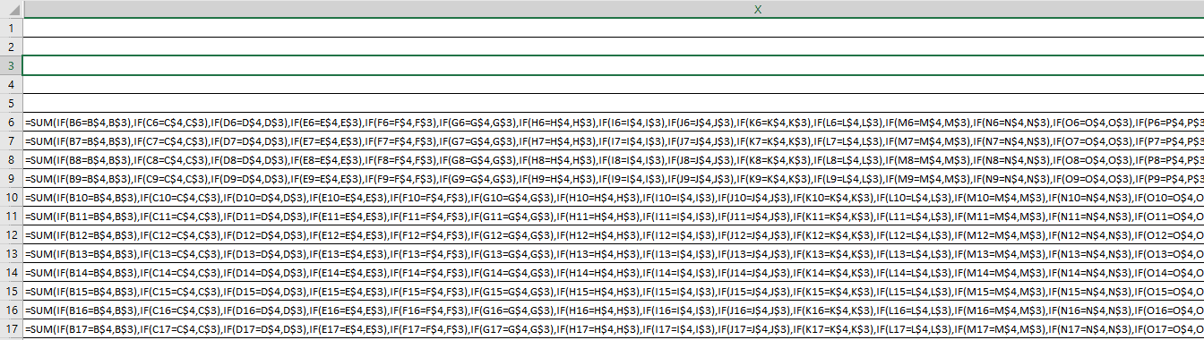
A little more complicated, here are the total points where each one is looking at cells matching to add the value found in row 3
Now lets start fresh, here I put in the one formula and spread it across the other cells, you can see only the first is accurate
Here is the formula side, this is what happens when you do not use the absolute reference ($) for these kinds of complicated formulas;
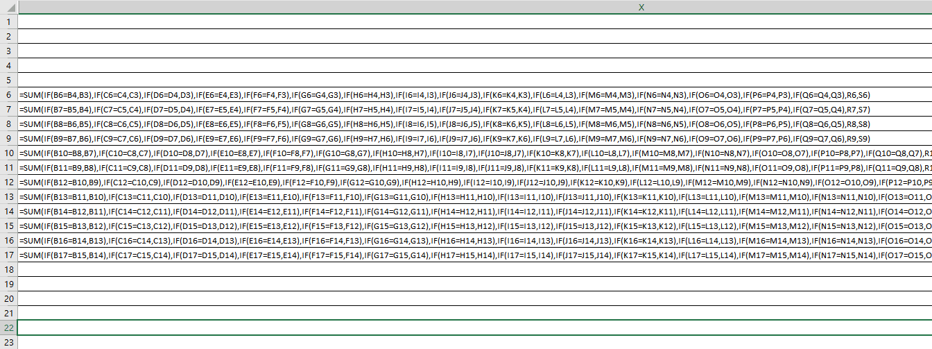
Notice it keeps counting the cells below, in pattern, now let me delete it all and go back to that first one and add the absolute reference ($);
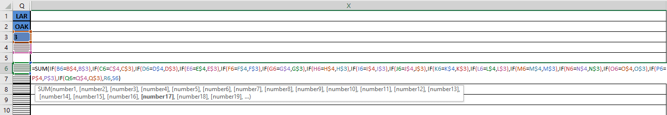
Now when I pull it down, I get the actual formula;
Here is the other end;
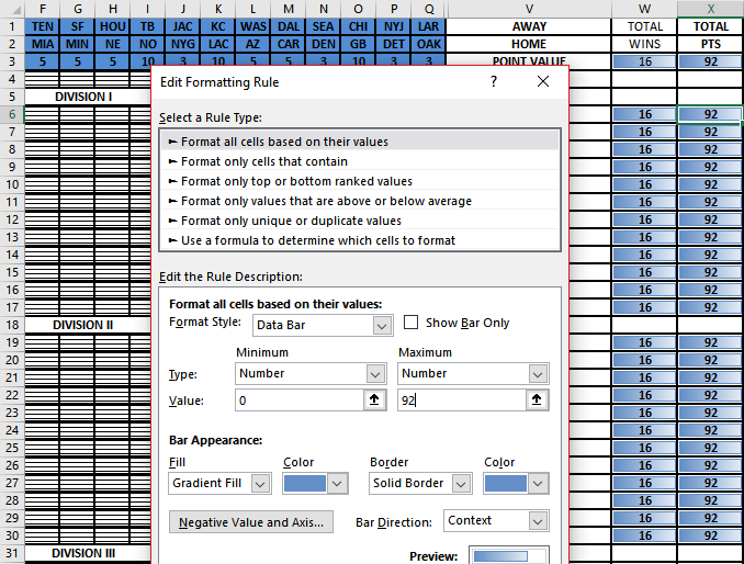
Now back to those data bars, we need to add rules for those;
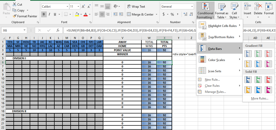
Under manage rules you can adjust the format style (Data bar) and adjust the number to minimum and maximum values. Here they were set 0 to 92, the most points you can get that week;
Now let’s fill in some winners to watch those bars in action;
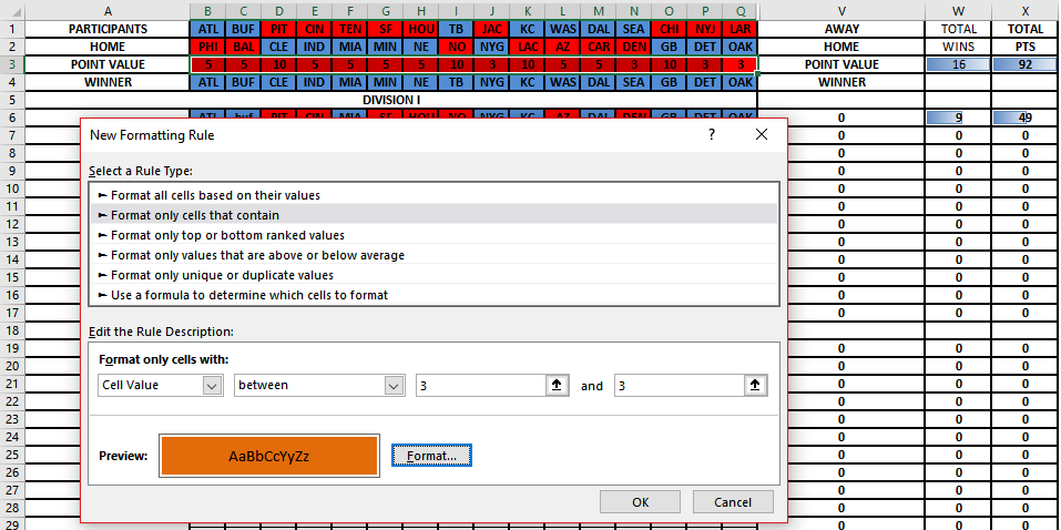
It was easier to add the rule of the “red for losers, blue for winners” with point value in tow but we want to set those different so we add more rules, this time I want the “Format only cells that contain”, and here I select “3” and fill it orange if 3 is shown.
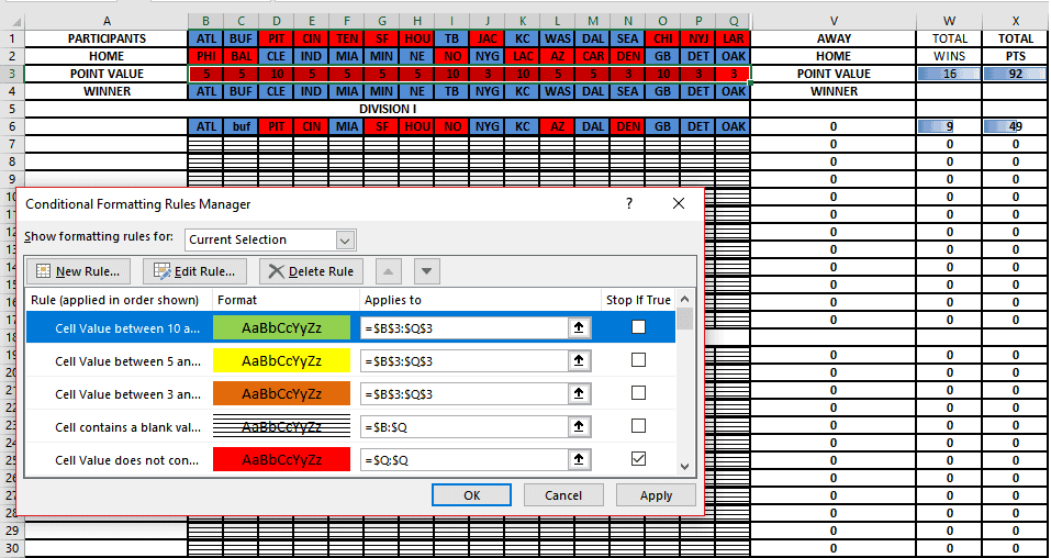
But I am not stopping there, I need to differentiate 5 and 10 as well so here are those rules;
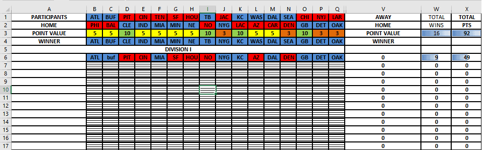
And the final results;
That’s it. When I did this formula the long way, it paid for itself in the time saved but had I known then, what I know now, it would have paid off much sooner.
Now you should be a little more comfortable and less intimidated by conditional formulas and formatting, flash filling, tables, and charts so go play with your new-found skills and feel free to contact me below or at Ben@eagleyeforum.com if you have any questions or suggestions.
Coming Soon…
For our last level, we will learn how to take tables further into pivot tables, how to make a macro, 3D map and timelines, and drop down lists.